
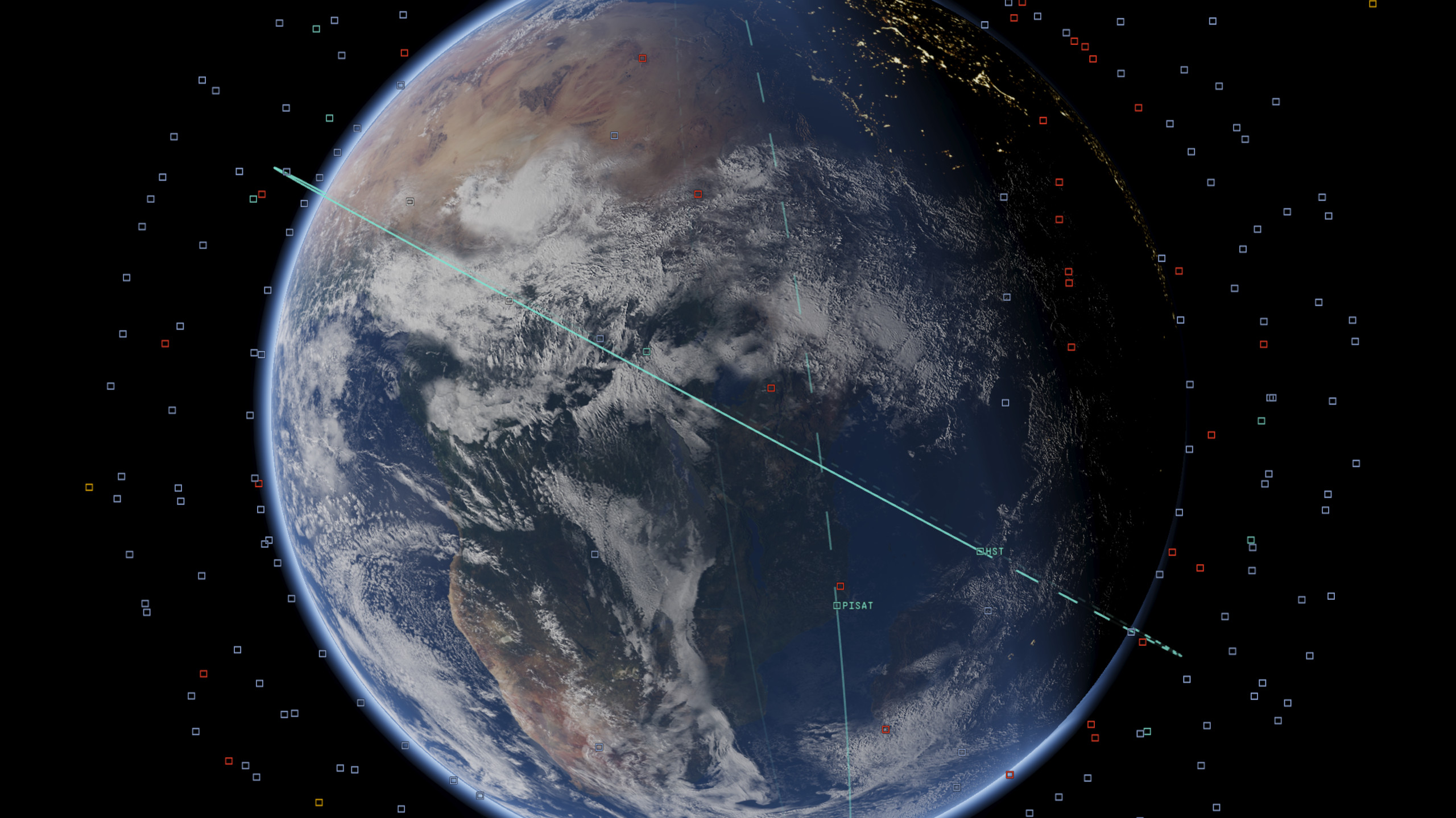
Above us, tens of thousands of human-made objects are moving around our Earth. Some are working satellites; others are rocket bodies, fragments of debris, or objects whose purpose is not publicly known. It is an environment that is both crowded and almost entirely invisible from the ground.
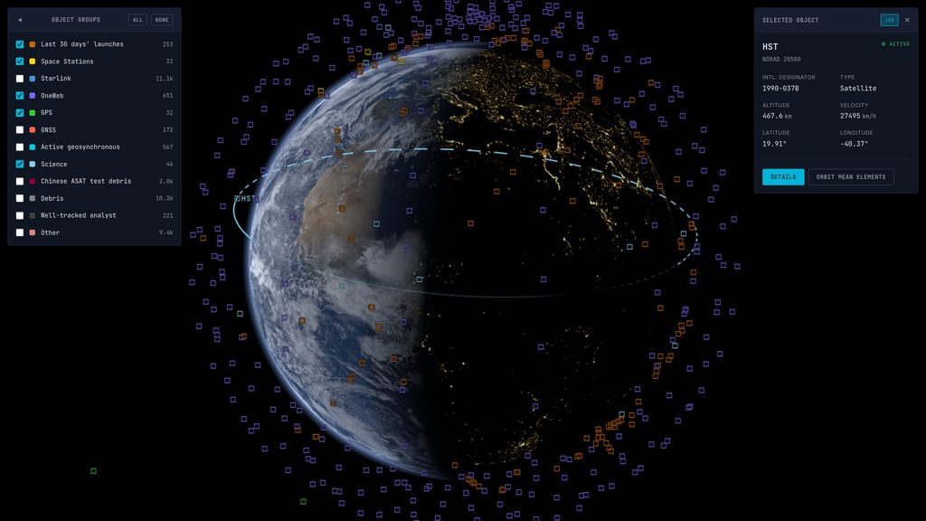
Apsis is a window into this environment: a browser-based visualisation of the objects in the public orbital catalogue, propagated to their current positions and rendered around a three-dimensional Earth.
If you are on a desktop PC or Mac with WebGPU support, you can try it at apsis.earth.
Why this exists
I developed Apsis as a way to exercise Pandora, my C++ and WebGPU engine, against a real-world problem rather than another gamedev-oriented project.
Orbital visualisation turned out to be a particularly useful endeavour. It combines a large and continuously changing dataset with a non-trivial numerical model, GPU compute, and a browser-based interface that needs to communicate with the underlying engine. These are all tightly interconnected, which makes the project both more useful and more interesting than a collection of isolated engine demos.
The world does not lack satellite visualisers. What interested me was building one around today’s catalogue scale and treating WebGPU (and particularly compute shaders) as a foundation rather than an optional enhancement.
As of 14 September 2026, the Apsis API returns 32,542 orbital objects. Of those, 253 are associated with launches from the preceding 30 days.
How it fits together
At a high level, Apsis has the following architecture:
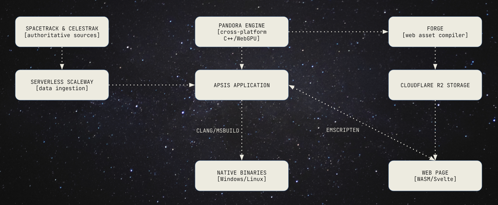
Space-Track is the authoritative source for the catalogue, orbital elements and associated metadata. CelesTrak plays a different role; Apsis uses its public group lists to classify objects into useful sets such as space stations, Starlink, OneWeb, GPS, science missions and the debris from the 2007 Chinese anti-satellite test. Other groups, such as all debris and launches from the last 30 days, are derived from the Space-Track metadata.
It is important to point out that this is not live telemetry. The source data consists of orbital element sets published by the tracking network – essentially parameters describing an orbit at a certain point in time – which Apsis then uses to estimate where each object should be at the current time.
Ideally I’d just use a few API endpoints and run everything client-side, but that’s not really possible: not only is this a large amount of data, but the data providers very explicitly ask people to cache as much as possible to reduce the strain on their servers. To achieve this, I’ve built a data ingestion service using Scaleway, a European cloud provider. Separate ingestion jobs fetch the data from Space-Track and CelesTrak and store it in a serverless PostgreSQL database.
A small Rust API, deployed as serverless functions, queries PostgreSQL and returns the orbital records and group membership as one JSON payload. The Apsis application downloads that data, creates an entity per catalogue entry, and builds the set of objects that should currently be propagated and displayed.
Apsis is built on top of a custom engine, Pandora, which is capable of deploying either native binaries or for web. Assets (e.g. the Earth’s textures) are built by Forge, and then uploaded to a Cloudflare R2 storage bucket. I’ll go into more details about this later in this post.
Finally, the user interface is done with Svelte and communicates with the application via Emscripten’s interop.
Propagating tens of thousands of orbits
The estimated position for the satellites is produced with SGP4 and its deep-space counterpart, SDP4. These are the standard general-perturbations models used with the public catalogue data from Space-Track. The near-Earth path includes effects such as the Earth’s oblateness and atmospheric drag; the deep-space path adds lunar-solar perturbations and resonance terms.
The implementation in Apsis was written from the published algorithms in Spacetrack Report #3 and the corrections in Revisiting Spacetrack Report #3. The test suite compares it against David Vallado’s reference implementation and published verification data.
Both SGP4 and SDP4 are complex, but remain cheap enough to evaluate for a very large number of objects on modern hardware, as long as that work is distributed. The simplest approach is to run every object on the main thread on the CPU: certainly doable, but the cost is prohibitive with the full dataset. For example, when targeting web via WASM rather than running native code we’re looking at 40ms per frame on my i7-14700K, which is far above the 16.6ms/frame required to hit 60FPS.
However, these propagation models have the advantage that they can be fully parallelised as the satellites are entirely independent from each other. This allows us to leverage the highest level of parallel processor we have – the GPU, via compute shaders.
For the current implementation in Apsis, the work is split between the CPU and GPU. Initialising an element set involves calculating a large collection of coefficients which remain fixed for the life of that data. Apsis performs that stage once on the CPU in double precision and when the visible roster changes, those coefficients are narrowed to 32-bit floats and uploaded to a WebGPU storage buffer. This is a limitation of WebGPU: at the time of writing, it doesn’t support 64-bit floats.
At the time of writing, WebGPU does not support 64-bit floats, so the propagation calculations are narrowed to 32-bit floats. Although the loss of precision adds up, comparing the outputs between 32-bit and 64-bit floating point calculations resulted in a position delta of less than 100 meters for the worst cases.
After that, the per-frame input is minimal: just one float per object, containing the number of minutes since that object’s epoch. A WGSL compute shader runs one invocation per visible object and writes its position, velocity and any propagation error to an output buffer.
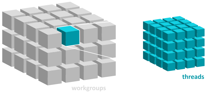
As WebGPU readback cannot block the browser, the result is asynchronous and a completed propagation is normally a couple of frames behind the dispatch. For our use case, this isn’t an issue: the movement remains smooth, and the visual position being a few frames delayed is not noticeable.
Once the result returns, the CPU converts the inertial coordinates into world space and derives latitude, longitude, altitude and speed for the selected-object panel. The Earth is oriented separately each frame using Greenwich Mean Sidereal Time. The renderer projects the visible objects into screen space, hides those behind the Earth, and batches their markers and labels into a dynamic vertex buffer. When more than 100 objects are visible, full names are limited to the selected and hovered objects to maintain legibility.
In a recent browser/wasm development capture on my RTX 5090, a view containing all 32,542 objects maintains 70 frames per second (limited by vsync), with the GPU propagation pass averaging roughly 0.15 ms. That was profiled on a high-end development machine and is of course not representative of consumer-grade hardware, but it demonstrates that the approach leaves room for the rest of the frame rather than spending the entire budget updating orbits.
Pandora: the engine underneath
Apsis is built on Pandora, a custom C++20 engine I have been developing over the past year. Pandora provides the WebGPU renderer, an EnTT-based entity-component system, resource and virtual-file-system layers, input, scene management and the platform lifecycle used by the application.
Pandora targets the browser through Emscripten and browser WebGPU, while native Windows and Linux builds use Dawn. WebGPU does not make Direct3D or Vulkan disappear; rather, it provides a common graphics API and one shader language across those targets rather than maintaining a separate rendering backend for each.
The browser is a first-class platform rather than a late port, and that affects more than rendering. For example, reading an asset from an SSD and downloading it over the network have very different failure modes and performance characteristics.
Pandora’s asset tool, Forge, compiles source assets ahead of time and produces a manifest containing their paths, sizes and content hashes. Native builds read those compiled assets from disk. Web builds request them by hash from object storage, verify them on arrival, and use the browser’s persistent fetch cache. Earth textures are stored as KTX2, preserving compressed assets and allowing Pandora to transcode compatible payloads for the formats supported by the GPU rather than downloading large uncompressed images.
The same resource interface sits above both implementations, abstracting away the underlying platform and enforcing asynchronous asset loading.
A Svelte shell around a C++ application
As mentioned before, the C++ application is compiled to WebAssembly, and Emscripten connects it to a WebGPU canvas. The same C++ code owns the scene, catalogue entities, propagation and rendering.
SvelteKit provides the static web application around that canvas: loading and error states, group filters, and the information panel for a selected object. C++ sends selection updates and group definitions to JavaScript callbacks; the Svelte controls call exported bindings when a filter changes. This bridging is done via Emscripten’s interop functionality.
I like this division because it lets each side do the work it is suited to: the simulation and rendering remain in the engine, while the surrounding interface remains ordinary reactive web UI. This means Pandora has no need to re-invent the wheel regarding implementing its own UI primitives, and only has to handle very limited text rendering.
Rendering Earth
The Earth is generated at runtime rather than loaded as a model: for Apsis’ use-case, there is no reason to download and load a model when one can be generated mathematically. The technique to create the geometry is simple, if somewhat counter-intuitive: we start with the six faces of a cube and subdivide them, then project them into an sphere:
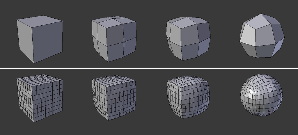
In Apsis’ case, it’s not a true sphere: Earth is an ellipsoid, with different semi-major and semi-minor axes (~6378km and ~6356km, respectively). This is the WGS84 reference ellipsoid.
This approach distributes geometry more evenly than a conventional latitude-longitude sphere while preserving the equirectangular texture mapping used by the source imagery. Additionally, by subdividing from a cube, future implementation of texture streaming and virtual texturing will be significantly easier.
The surface currently uses five 8192×4096 source maps: colour, city lights, ocean/specular mask, normals and cloud coverage. The daytime colour map comes from NASA Earth Observatory’s Blue Marble: Next Generation. The other maps are credited to Solar System Scope and are derived from NASA data. They are compiled into KTX2 assets for deployment rather than shipped as the original images.
The planet shader combines directional sunlight, normal-mapped terrain, Fresnel ocean reflections, city lights and a cloud layer which moves over the surface. The cloud layer both casts shadows and self-shadows: it is a subtle effect, but without it the clouds look unnaturally flat.

The atmosphere is rendering in a separate pass using an adaptation of Sean O’Neil’s scattering model from GPU Gems 2, ray-marching 16 samples per pixel and combining Rayleigh and Mie scattering. This is also one of the visibly unfinished parts of the project. My implementation of O’Neil’s approximation tends to saturate before producing as much orange around the terminator as I want, so we don’t get dramatic sunsets. Although various tweaks have improved it substantially, I plan to eventually replace it with a more complete scattering model.
An ongoing project
Apsis is usable, but it is not finished yet – there is still a great deal to do.
In addition to general polish, the following major items are on the wishlist:
- The selected-object panel currently only exposes the values produced directly by propagation and a small amount of metadata. I want to enrich it with launch details and country of origin, as well as additional context from The Space Devs.
- At the moment the background is solid black, with only the sun being visible in the distance. I would like to add a proper starfield based on real catalogue data.
- Although a major body of work, I would like to add time controls and a timelapse mode. This can’t be done solely from the current propagation data: it doesn’t contain objects that have already decayed, and the SGP4 model accumulates errors quickly. Anything more than a few days old is speculative at best, and trying to propagate back to 1958 would be completely wrong. However, being able to see a timelapse since Sputnik 1 was launched until the present day would be incredible.
Apsis began as a way to test a custom engine, but it has become an excellent way to learn everything from reference frames and numerical validation to content-addressed assets and the awkward boundary between WebAssembly and browser UI. More importantly, it turns an abstract catalogue into something we can see, a window to the continually moving environment above us.
Try it at apsis.earth.
The source is available at github.com/solace-10/apsis, and Pandora is available at github.com/solace-10/pandora.